A decision tree is a popular supervised machine learning algorithm used for both classification and regression tasks. It works with categorical as well as continuous output variables and is widely used due to its simplicity, interpretability and strong performance on structured data.
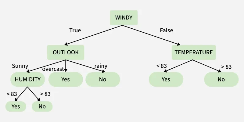
In the above figure, a decision tree is a flowchart-like structure with a root node (WINDY), internal nodes (OUTLOOK, TEMPERATURE) for attribute tests and leaf nodes for final decisions. The branches show the possible outcomes of each test. A Decision Tree follows a tree-like structure where:
- Nodes represent decisions or feature tests
- Branches represent outcomes of those decisions
- Leaf nodes represent final predictions or class labels
The tree is constructed by recursively splitting the dataset based on the feature that provides the maximum information gain or minimum impurity.
How Decision Trees Work
Decision Trees work by selecting the best attribute at each step to split the data. This selection is based on statistical metrics that measure data impurity or uncertainty.
- Start with the full dataset as the root node.
- Select the best feature using a splitting criterion.
- Split the dataset into subsets.
- Repeat the process recursively until stopping conditions are met.
- Assign class labels at leaf nodes.
Splitting Criteria in Decision Trees
Decision Trees select the best attributes for splits using metrics like Gini Index, Entropy and Information Gain helping decide the root and internal nodes. Entropy measures dataset impurity, guiding the tree to choose splits that reduce uncertainty.
1. Gini Index
Measures the probability of misclassifying a randomly chosen element lower values are better.
\text{Gini Index} = 1 - \sum_{j} p_j^2
where
2. Entropy
Quantifies the uncertainty or impurity in a dataset higher entropy means more disorder.
H(x) = - \sum_{i=1}^{N} p(x_i) \log_2 p(x_i)
where
x_i : possible value of a variablep(x_i) : probability ofx_i
3. Information Gain
Measures the reduction in entropy achieved by splitting data on an attribute higher gain is preferred.
IG(S, A) = H(S) - \sum_{v \in \text{Values}(A)} \frac{|S_v|}{|S|} H(S_v)
H(S) : Entropy before split.H(S_v) : Entropy of subset after split.IG(S, A) : Reduction in entropy from splitting on A.
Step By Step Implementation
Here we implement Decision Tree classifiers on the Balance Scale dataset, evaluate their performance and visualize the resulting trees.
Step 1: Install Libraries and Import Dependencies
- Import pandas, numpy for data handling and matplotlib for plotting.
- import scikit learn for Decision Tree implementation
- Import metrics for evaluating model performance
pip install -U scikit-learn
import numpy as np
import pandas as pd
from sklearn.metrics import confusion_matrix, accuracy_score, classification_report
from sklearn.model_selection import train_test_split
from sklearn.tree import DecisionTreeClassifier, plot_tree
import matplotlib.pyplot as plt
Step 2: Import Dataset
- Load the dataset from the UCI repository.
- Display dataset length, shape and first few rows.
- Returns the dataset for further processing.
def importdata():
    url = "https://archive.ics.uci.edu/static/public/12/data.csv"
    balance_data = pd.read_csv(url, header=0)
    print("Dataset Length:", len(balance_data))
    print("Dataset Shape:", balance_data.shape)
    print("Dataset Head:\n", balance_data.head())
    return balance_data
Step 3: Split Dataset into Features and Labels
- Separate input features (X) and target labels (Y).
- Split data into training and testing sets.
- Return both the complete dataset and split sets for modeling.
def splitdataset(balance_data):
    X = balance_data.iloc[:, 1:5].values
    Y = balance_data.iloc[:, 0].values
    X_train, X_test, y_train, y_test = train_test_split(X, Y, test_size=0.3, random_state=100)
    return X, Y, X_train, X_test, y_train, y_test
Step 4: Train Decision Tree Using Gini Index
- Initialize DecisionTreeClassifier with gini criterion.
- Set max_depth and min_samples_leaf to control tree complexity.
- Fit the model on training data and return the trained classifier.
def train_using_gini(X_train, y_train):
    clf_gini = DecisionTreeClassifier(criterion="gini", random_state=100, max_depth=3, min_samples_leaf=5)
    clf_gini.fit(X_train, y_train)
    return clf_gini
Step 5: Train Decision Tree Using Entropy
- Initialize classifier with entropy criterion.
- Same depth and leaf settings to compare with Gini.
- Fit the model on training data and return the trained classifier.
def train_using_entropy(X_train, y_train):
    clf_entropy = DecisionTreeClassifier(criterion="entropy", random_state=100, max_depth=3, min_samples_leaf=5)
    clf_entropy.fit(X_train, y_train)
    return clf_entropy
Step 6: Make Predictions
Use the trained classifier to predict target labels for the test set.
def prediction(X_test, clf_object):
    y_pred = clf_object.predict(X_test)
    print("Predicted Values:\n", y_pred)
    return y_pred
Step 7: Evaluate Model Accuracy
- Calculate and display the confusion matrix.
- Compute accuracy score.
- Show detailed classification report including precision, recall and F1-score.
def cal_accuracy(y_test, y_pred):
    print("\nConfusion Matrix:\n", confusion_matrix(y_test, y_pred))
    print("\nAccuracy:", accuracy_score(y_test, y_pred) * 100)
    print("\nClassification Report:\n", classification_report(y_test, y_pred))
Step 8: Visualize the Decision Tree
- Plot the trained decision tree using matplotlib.
- Include feature names and class names for better readability.
def plot_decision_tree(clf_object, feature_names, class_names):
    plt.figure(figsize=(15, 10))
    plot_tree(clf_object, filled=True, feature_names=feature_names, class_names=class_names, rounded=True)
    plt.show()
Step 9: Train, Predict and Evaluate Models
- Load and split the dataset into training and testing sets.
- Train classifiers using Gini and Entropy criteria.
- Make predictions on the test set and evaluate accuracy using confusion matrix, accuracy score and classification report.
if __name__ == "__main__":

    data = importdata()
    X, Y, X_train, X_test, y_train, y_test = splitdataset(data)


    print("\n----- Training Using Gini -----")
    clf_gini = train_using_gini(X_train, y_train)
    y_pred_gini = prediction(X_test, clf_gini)
    cal_accuracy(y_test, y_pred_gini)


    print("\n----- Training Using Entropy -----")
    clf_entropy = train_using_entropy(X_train, y_train)
    y_pred_entropy = prediction(X_test, clf_entropy)
    cal_accuracy(y_test, y_pred_entropy)
Output:
The Decision Tree trained using Gini and Entropy achieves around 73% and 71% accuracy respectively, showing similar performance. Both models classify L and R classes reasonably well, but fail to correctly predict the B class, likely due to class imbalance.
Step 10: Visualize Decision Trees
Plot both Gini and Entropy trained decision trees using matplotlib.
plot_decision_tree(clf_gini, ['X1', 'X2', 'X3', 'X4'], ['L', 'B', 'R'])

plot_decision_tree(clf_entropy, ['X1', 'X2', 'X3', 'X4'], ['L', 'B', 'R'])
Output:
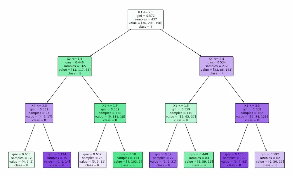
Gini Index Tree: The tree splits features based on minimizing the Gini impurity focusing on how often a randomly chosen element would be incorrectly classified. It aims for pure nodes with minimal class mixing.
.webp)
Entropy Tree: The tree splits features based on information gain (entropy reduction), selecting splits that maximize the reduction in uncertainty about the class labels. It tends to create balanced splits that reduce overall disorder.
You can download full code from here
Applications
- Used for classification tasks such as spam detection and fraud detection.
- Applied in regression problems like house price prediction.
- Helps in medical diagnosis and disease prediction.
- Used in credit risk analysis and loan approval systems.
- Useful for feature selection and customer segmentation.
Advantages
- Easy to understand, interpret and visualize.
- Works with both numerical and categorical data.
- Requires little or no data preprocessing.
- Does not assume any underlying data distribution.
- Provides feature importance for model interpretation.
Limitations
- Prone to overfitting, especially with deep trees.
- Sensitive to small changes in training data.
- Performs poorly on imbalanced datasets.
- Lower accuracy compared to ensemble models.
- Uses greedy splitting which may not be globally optimal.