A Decision Tree Regressor is used to predict continuous values such as prices or scores using a tree-like structure. It splits the data into smaller groups based on simple rules derived from input features, helping reduce prediction errors. At the end of each branch, called a leaf node, the model outputs a value, i.e., usually the average of that group.
For example, to predict house prices using features like size, location, and age, the tree may first split by location, then by size and finally by age. Let’s implement it:
Step 1: Importing the required libraries
We will import the following libraries.
- NumPy: For numerical computations and array handling
- Matplotlib: For plotting graphs and visualizations
- We import different modules from scikit-learn for various tasks such as modeling, data splitting, tree visualization and performance evaluation.
import numpy as np
import matplotlib.pyplot as plt
from sklearn.tree import DecisionTreeRegressor, export_text
from sklearn.model_selection import train_test_split
from sklearn.metrics import mean_squared_error
Step 2: Creating a Sample Dataset
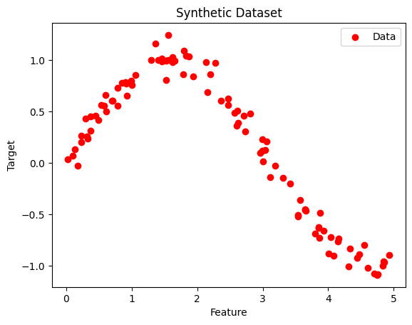
Here we create a synthetic dataset using numpy library, where the feature values X are randomly sampled and sorted between 0 and 5 and the target y is a noisy sine function of X. The scatter plot visualizes the data points, showing how the target values vary with the feature.
np.random.seed(42)
X = np.sort(5 * np.random.rand(100, 1), axis=0)
y = np.sin(X).ravel() + np.random.normal(0, 0.1, X.shape[0])

plt.scatter(X, y, color='red', label='Data')
plt.title("Synthetic Dataset")
plt.xlabel("Feature")
plt.ylabel("Target")
plt.legend()
plt.show()
Output:
Step 3: Splitting the Dataset
We split the dataset into train and test dataset using the train_test_split function into the ratio of 70% training and 30% testing. We also set a random_state=42 to ensure reproducibility.
X_train, X_test, y_train, y_test = train_test_split(X, y, test_size=0.3, random_state=42)
Step 4: Initializing the Decision Tree Regressor
Here we used DecisionTreeRegressor method from Sklearn python library to implement Decision Tree Regression. We also define the max_depth as 4 which controls the maximum levels a tree can reach , controlling model complexity.
regressor = DecisionTreeRegressor(max_depth=4, random_state=42)
Step 5: Fitting Decision Tree Regressor Model
We fit our model using the .fit() method on the X_train and y_train, so that the model can learn the relationships between different variables.
regressor.fit(X_train, y_train)
Output:
DecisionTreeRegressor(max_depth=4, random_state=42)
Step 6: Predicting a New Value
We will now predict a new value using our trained model using the predict() function. After that we also calculated the mean squared error (MSE) to check how accurate is our predicted value from the actual value , telling how well the model fits to our training data.
y_pred = regressor.predict(X_test)

mse = mean_squared_error(y_test, y_pred)
print(f"Mean Squared Error: {mse:.4f}")
Output:
Mean Squared Error: 0.0151
Step 7: Visualizing the result
We will visualise how the model makes predictions to see how well the decision tree fits the data and captures the underlying pattern, especially showing how the predictions change in step-like segments based on the tree’s splits.
X_grid = np.arange(min(X), max(X), 0.01)[:, np.newaxis]
y_grid_pred = regressor.predict(X_grid)

plt.figure(figsize=(10, 6))
plt.scatter(X, y, color='red', label='Data')
plt.plot(X_grid, y_grid_pred, color='blue', label='Model Prediction')
plt.title("Decision Tree Regression")
plt.xlabel("Feature")
plt.ylabel("Target")
plt.legend()
plt.show()
Output:

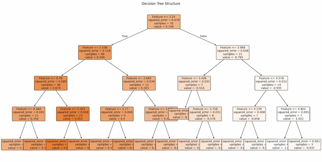
Step 8: Export and Show the Tree Structure below
For better understanding we used plot_tree to visualize the structure of the decision tree to understand how the model splits the feature space, showing the decision rules at each node and how the tree partitions the data to make predictions.
from sklearn.tree import plot_tree

plt.figure(figsize=(20, 10))
plot_tree(
    regressor,
    feature_names=["Feature"],
    filled=True,
    rounded=True,
    fontsize=10
)
plt.title("Decision Tree Structure")
plt.show()
Output:
Decision Tree Regression is used for predicting continuous values effectively capturing non-linear patterns in data. Its tree-based structure makes model interpretability easy as we can tell why a decision was made and why we get this specific output. This information can further be used to fine tune model based on it flow of working.